MAT 350 PROJECT ONE GUIDELINES AND RUBRIC / MAT 350 PROJECT ONE TEMPLATE
MAT 350 Project One Template
MAT350: Applied Linear Algebra
Problem 1
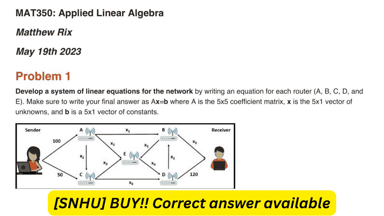
Develop a system of linear equations for the network by writing an equation for each router (A, B, C, D, and E). Make sure to write your final answer as Ax=b where A is the 5×5 coefficient matrix, x is the 5×1 vector of unknowns, and b is a 5×1 vector of constants.
Solution:
System of linear equations:
The input was set equal to the output and then equations were simplified to put all variables on the left. Router A recieves 100 and outputs x1 once and x2 twice:
x1 + 2x2 = 100
Router B recieves x1 and x2 and outputs x3 once and x5 once:
x3 + x5 = x1 + x2
-x1 – x2 + x3 + x5 = 0
Router C recieves 100 and x2 while outputing x3 and x5:
-x2 + x3 + x5 = 50
Router D recieves x5 and x4 and outputs x2 and 120:
x4 + x5 = 120 + x2
-x2 + x4 + x5 = 120
Router E recieves x2, x3, and x5 and outputs x4:
x4 = x2 + x3 + x5 x2 + x3 – x4 + x5 = 0
Problem 2
Use MATLAB to construct the augmented matrix [A b] and then perform row reduction using the rref() function. Write out your reduced matrix and identify the free and basic variables of the system.
Solution:
A = 5×5
| 1 | 2 | 0 | 0 | 0 |
| -1 | -1 | 1 | 0 | 1 |
| 0 | -1 | 1 | 0 | 1 |
| 0 | -1 | 0 | 1 | 1 |
| 0 | 1 | 1 | -1 | 1 |
b = 5×1
100
0
50
120
0
Ab = 5×6
| 1 | 2 | 0 | 0 | 0 | 100 |
| -1 | -1 | 1 | 0 | 1 | 0 |
| 0 | -1 | 1 | 0 | 1 | 50 |
| 0 | -1 | 0 | 1 | 1 | 120 |
| 0 | 1 | 1 | -1 | 1 | 0 |
rowreducedAb = 5×6
| 1 | 0 | 0 | 0 | 0 | 50 |
| 0 | 1 | 0 | 0 | 0 | 25 |
| 0 | 0 | 1 | 0 | 0 | 30 |
| 0 | 0 | 0 | 1 | 0 | 100 |
| 0 | 0 | 0 | 0 | 1 | 45 |
A basic variable correspnds to the variable in one of the matrix’s pivot columns and free variables cannot exist within a pivot column. Every column is a pivot column, therefore, there are no free variables and the columns x1, x2, x3, x4, and x5 are basic variables.
Problem 3
Use MATLAB to compute the LU decomposition of A, i.e., find A = LU. For this decomposition, find the transformed set of equations Ly = b, where y = Ux. Solve the system of equations Ly = b for the unknown vector y.
Solution:
| L = 5×5 | ||||||
| 1.0000 | 0 | 0 | 0 | 0 | ||
| -1.0000 | 1.0000 | 0 | 0 | 0 | ||
| 0 | -1.0000 | 1.0000 | 0 | 0 | ||
| 0 | -1.0000 | 0.5000 | 1.0000 | 0 | ||
| 0 | 1.0000 | 0 | -1.0000 | 1.0000 | ||
| U = 5×5 | ||||||
| 1 | 2 | 0 | 0 | 0 | ||
| 0 | 1 | 1 | 0 | 1 | ||
| 0 | 0 | 2 | 0 | 2 | ||
| 0 | 0 | 0 | 1 | 1 | ||
| 0 | 0 | 0 | 0 | 1 | ||
y = 5×1
100
100
150
145
45
Problem 4
Use MATLAB to compute the inverse of U using the inv() function.
Solution:
ans = 5×5
| 1.0000 | -2.0000 | 1.0000 | 0 | 0 |
| 0 | 1.0000 | -0.5000 | 0 | 0 |
| 0 | 0 | 0.5000 | 0 | -1.0000 |
| 0 | 0 | 0 | 1.0000 | -1.0000 |
| 0 | 0 | 0 | 0 | 1.0000 |
Problem 5
Compute the solution to the original system of equations by transforming y into x, i.e., compute x = inv(U)y.
Solution:
x = 5×1
50
25
30
100
45
Problem 6
Check your answer for using Cramer’s Rule. Use MATLAB to compute the required determinants using the det() function.
Solution:
A1 = 5×5
| 1 | 2 | 0 | 0 | 0 | |
| -1 | -1 | 1 | 0 | 1 | |
| 0 | -1 | 1 | 0 | 1 | |
| 0 | -1 | 0 | 1 | 1 | |
| 0 | 1 | 1 | -1 | 1 | |
| % Replace the appropriate variable | |||||
| A1(:,1) | = | b | |||
| A1 = 5×5
100 |
2 |
0 |
0 |
0 |
|
| 0 | -1 | 1 | 0 | 1 | |
| 50 | -1 | 1 | 0 | 1 | |
| 120 | -1 | 0 | 1 | 1 | |
| 0 | 1 | 1 | -1 | 1 | |
x1 = 50
Problem 7
The Project One Table Template, provided in the Project One Supporting Materials section in Brightspace, shows the recommended throughput capacity of each link in the network. Put your solution for the system of equations in the third column so it can be easily compared to the maximum capacity in the second column. In the fourth column of the table, provide recommendations for how the network should be modified based on your network throughput analysis findings. The modification options can be No Change, Remove Link, or Upgrade Link. In the final column, explain how you arrived at your recommendation.
Solution:
Fill out the table in the original project document and export your table as an image. Then, use the Insert tab in the MATLAB editor to insert your table as an image.
I had to make my own table in a libre file document since SNHU’s student license doesn’t extend to editing word documents on a MacOS.
Related; MAT350 8.5 MATLAB: Least Squares Approximation.
Order This Paper

Reviews
There are no reviews yet.